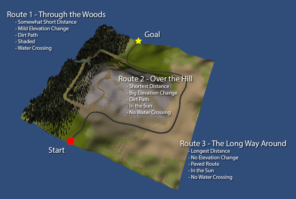
This example demonstrates using an OWA operator to aggregate path costs along different routes as a way of implementing bounded rationality. Consider the example in the figure below. There are three different routes that an agent can take to reach the goal. Each route has different tradeoffs and agents with different preferences could favor different routes.

In the interactive example below, the three routes are displayed on a grid where each grid cell is assigned properties from the environment. You can toggle the individual feature layers using the radio selections. Below the grid are a set of sliders representing the agent's preferences for each of the feature types. The OWA weights used for aggregation are at the bottom.
The right side of the figure shows the individual step costs for each path as evaluated by the agent. The F-values show the segment's features and the A-values show the agents assessment of each feature. The assessments are sorted in decreasing order and multiplied with the OWA weights to give the segment cost. The total cost of the path is shown at the top, and the relative path costs are plotted next to the figure.
By changing the agent's preferences and OWA weights, we can see how the three different paths are evaluated. Can you find parameter settings that make each of the three paths the most desirable (lowest cost)?
| R1 | R2 | R3 |
Agent Profile |
||
|---|---|---|
| Slope Influence | ||
| Path Type Influence | ||
| Water Crossing Influence | ||
| Unshaded Influence | ||